Predicting Occupancy of a Room, Part 1
I decided to take on the Occupancy dataset from UCI Machine Learning. With this dataset, I wanted to accomplish 2 tasks:
- Predict the occupancy of a room given parameters.
- Conduct Time Series Analysis to forecast the parameters and predict occupancy.
The tasks may sound similar, but they’re actually different. The first one does not take the time into account, but rather uses the parameters or a subset of the parameters given (Light, Humidity, Temperature, CO2, etc.) to predict the occupancy of the room (binary -> 0 or 1). The second task actually does take the time into account, and forecasts the individual parameters to predict the occupancy of the room at specific times where the parameters were forecast.
In this post, I am going to show how I tackle the first task. This example uses Python 3. First, import the required modules and packages:
import numpy as np
import pandas as pd
from sklearn.metrics import accuracy_score, plot_confusion_matrix
import matplotlib.pyplot as plt
import seaborn as sns
from sklearn.linear_model import LogisticRegression
from sklearn.neighbors import KNeighborsClassifier
from sklearn.naive_bayes import GaussianNB
from sklearn.neural_network import MLPClassifier
from sklearn import svm
from sklearn.feature_selection import SelectKBest
from sklearn.feature_selection import f_classif
from sklearn import preprocessing
from sklearn.tree import DecisionTreeClassifier, export_graphviz,plot_tree
from sklearn.ensemble import RandomForestClassifier
from statsmodels.tsa.seasonal import seasonal_decompose
from statsmodels.tsa.stattools import adfuller
from statsmodels.tsa.stattools import grangercausalitytests
from fbprophet import Prophet
import warnings
warnings.filterwarnings('ignore')
%matplotlib inline
plt.rcParams['figure.figsize'] = [10.0, 6.0]
Then, read in the data:
# Read in data
df_train = pd.read_csv('train_data.txt')
df_val = pd.read_csv('validation_data.txt')
Explore the data:
# Explore data
df_train.head()
| date | Temperature | Humidity | Light | CO2 | HumidityRatio | Occupancy | |
|---|---|---|---|---|---|---|---|
| 1 | 2015-02-04 17:51:00 | 23.18 | 27.2720 | 426.0 | 721.25 | 0.004793 | 1 |
| 2 | 2015-02-04 17:51:59 | 23.15 | 27.2675 | 429.5 | 714.00 | 0.004783 | 1 |
| 3 | 2015-02-04 17:53:00 | 23.15 | 27.2450 | 426.0 | 713.50 | 0.004779 | 1 |
| 4 | 2015-02-04 17:54:00 | 23.15 | 27.2000 | 426.0 | 708.25 | 0.004772 | 1 |
| 5 | 2015-02-04 17:55:00 | 23.10 | 27.2000 | 426.0 | 704.50 | 0.004757 | 1 |
df_train.tail()
| date | Temperature | Humidity | Light | CO2 | HumidityRatio | Occupancy | |
|---|---|---|---|---|---|---|---|
| 8139 | 2015-02-10 09:29:00 | 21.05 | 36.0975 | 433.0 | 787.250000 | 0.005579 | 1 |
| 8140 | 2015-02-10 09:29:59 | 21.05 | 35.9950 | 433.0 | 789.500000 | 0.005563 | 1 |
| 8141 | 2015-02-10 09:30:59 | 21.10 | 36.0950 | 433.0 | 798.500000 | 0.005596 | 1 |
| 8142 | 2015-02-10 09:32:00 | 21.10 | 36.2600 | 433.0 | 820.333333 | 0.005621 | 1 |
| 8143 | 2015-02-10 09:33:00 | 21.10 | 36.2000 | 447.0 | 821.000000 | 0.005612 | 1 |
Data seems to be ordered by date and time and appropriate for time series analysis. Time intervals seem to be about every minute. Dates are from 2015-02-04 to 2015-02-10 (6 days).
df_train.info()
<class 'pandas.core.frame.DataFrame'>
Int64Index: 8143 entries, 1 to 8143
Data columns (total 7 columns):
date             8143 non-null object
Temperature      8143 non-null float64
Humidity         8143 non-null float64
Light            8143 non-null float64
CO2              8143 non-null float64
HumidityRatio    8143 non-null float64
Occupancy        8143 non-null int64
dtypes: float64(5), int64(1), object(1)
memory usage: 508.9+ KB
There are no null values in the training data. May need to convert date to datetime object. Occupancy is the only int type.
df_train.describe()
| Temperature | Humidity | Light | CO2 | HumidityRatio | Occupancy | |
|---|---|---|---|---|---|---|
| count | 8143.000000 | 8143.000000 | 8143.000000 | 8143.000000 | 8143.000000 | 8143.000000 |
| mean | 20.619084 | 25.731507 | 119.519375 | 606.546243 | 0.003863 | 0.212330 |
| std | 1.016916 | 5.531211 | 194.755805 | 314.320877 | 0.000852 | 0.408982 |
| min | 19.000000 | 16.745000 | 0.000000 | 412.750000 | 0.002674 | 0.000000 |
| 25% | 19.700000 | 20.200000 | 0.000000 | 439.000000 | 0.003078 | 0.000000 |
| 50% | 20.390000 | 26.222500 | 0.000000 | 453.500000 | 0.003801 | 0.000000 |
| 75% | 21.390000 | 30.533333 | 256.375000 | 638.833333 | 0.004352 | 0.000000 |
| max | 23.180000 | 39.117500 | 1546.333333 | 2028.500000 | 0.006476 | 1.000000 |
Occupancy seems to be binary: either 0 or 1. Assume 1 means occupied, and 0 means unoccupied.
# Convert date column to datetime object
df_train['date'] = pd.to_datetime(df_train['date'])
# Verify changed datatype for date
df_train.dtypes
date             datetime64[ns]
Temperature             float64
Humidity                float64
Light                   float64
CO2                     float64
HumidityRatio           float64
Occupancy                 int64
dtype: object
Date values are either at :00 or :59 seconds. Round all to nearest minute.
# Set date to index and round to nearest minute for time series analysis
df_train = df_train.set_index('date')
df_train.index = df_train.index.round('min')
df_train.head()
| Temperature | Humidity | Light | CO2 | HumidityRatio | Occupancy | |
|---|---|---|---|---|---|---|
| date | ||||||
| 2015-02-04 17:51:00 | 23.18 | 27.2720 | 426.0 | 721.25 | 0.004793 | 1 |
| 2015-02-04 17:52:00 | 23.15 | 27.2675 | 429.5 | 714.00 | 0.004783 | 1 |
| 2015-02-04 17:53:00 | 23.15 | 27.2450 | 426.0 | 713.50 | 0.004779 | 1 |
| 2015-02-04 17:54:00 | 23.15 | 27.2000 | 426.0 | 708.25 | 0.004772 | 1 |
| 2015-02-04 17:55:00 | 23.10 | 27.2000 | 426.0 | 704.50 | 0.004757 | 1 |
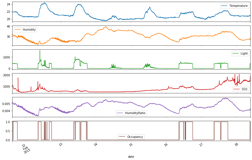
pd.plotting.register_matplotlib_converters()
# Plot all columns vs. date
df_train.plot(subplots=True, figsize=(15,10))
plt.show()
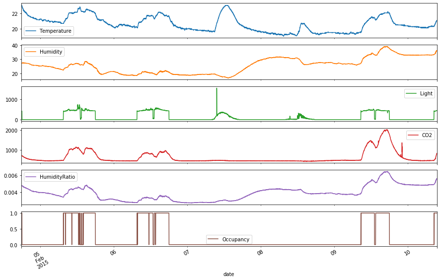
There appears to be some correlation between the variables, which can be seen from when the peaks occur. The occupancy seems less correlated to Humidity than it does with Light and CO2. Light seems to be the most important factor, since there are dips in the occupancy that coincide with dips in Light. There seems to be periodicity in the occupancy, where the occupancy can be 1 during “normal working hours” (i.e., 9am-6pm). However, there was no occupancy on 2 consecutive dates, 2015-02-07 and 2015-02-08. Perhaps those dates were the weekend, which indicates conditional seasonality. For those 2 dates, the CO2 levels were also very low with no peaks. Since the date range is small, assume no overall underlying trends in the variables. There also seems to be a high outlier in the Light data, with the value of 1546.3 within the day of 2015-02-07.
Check for Seasonality in parameters
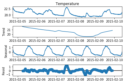
# Perform seasonality decomposition for Temperature, period = 1 day
seas_d = seasonal_decompose(df_train['Temperature'], period = (60*24))
fig=seas_d.plot()
fig.set_figheight(4)
plt.show()
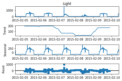
# Perform seasonality decomposition for Light, period = 1 day
seas_d = seasonal_decompose(df_train['Light'], period = (60*24))
fig=seas_d.plot()
fig.set_figheight(4)
plt.show()
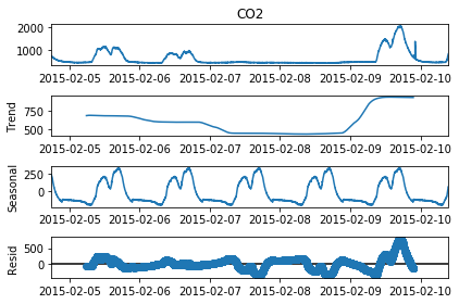
# Perform seasonality decomposition for CO2, period = 1 day
seas_d = seasonal_decompose(df_train['CO2'], period = (60*24))
fig=seas_d.plot()
fig.set_figheight(4)
plt.show()
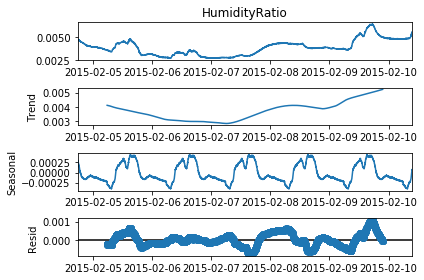
# Perform seasonality decomposition for HumidityRatio, period = 1 day
seas_d = seasonal_decompose(df_train['HumidityRatio'], period = (60*24))
fig=seas_d.plot()
fig.set_figheight(4)
plt.show()
Perform Granger Causality Tests
# Examine Temperature causing Occupancy
print(grangercausalitytests(df_train[['Occupancy', 'Temperature']], maxlag=4))
Granger Causality
number of lags (no zero) 1
ssr based F test:         F=10.5156 , p=0.0012  , df_denom=8139, df_num=1
ssr based chi2 test:   chi2=10.5195 , p=0.0012  , df=1
likelihood ratio test: chi2=10.5127 , p=0.0012  , df=1
parameter F test:         F=10.5156 , p=0.0012  , df_denom=8139, df_num=1

Granger Causality
number of lags (no zero) 2
ssr based F test:         F=3.5933  , p=0.0276  , df_denom=8136, df_num=2
ssr based chi2 test:   chi2=7.1910  , p=0.0274  , df=2
likelihood ratio test: chi2=7.1878  , p=0.0275  , df=2
parameter F test:         F=3.5933  , p=0.0276  , df_denom=8136, df_num=2

Granger Causality
number of lags (no zero) 3
ssr based F test:         F=1.1512  , p=0.3269  , df_denom=8133, df_num=3
ssr based chi2 test:   chi2=3.4566  , p=0.3264  , df=3
likelihood ratio test: chi2=3.4559  , p=0.3265  , df=3
parameter F test:         F=1.1512  , p=0.3269  , df_denom=8133, df_num=3

Granger Causality
number of lags (no zero) 4
ssr based F test:         F=0.6326  , p=0.6392  , df_denom=8130, df_num=4
ssr based chi2 test:   chi2=2.5331  , p=0.6387  , df=4
likelihood ratio test: chi2=2.5327  , p=0.6388  , df=4
parameter F test:         F=0.6326  , p=0.6392  , df_denom=8130, df_num=4
{1: ({'ssr_ftest': (10.515600218091105, 0.0011884805851629405, 8139.0, 1), 'ssr_chi2test': (10.51947622259464, 0.0011812295962018446, 1), 'lrtest': (10.512686480680713, 0.00118557768661934, 1), 'params_ftest': (10.515600218094972, 0.0011884805851604175, 8139.0, 1.0)}, [<statsmodels.regression.linear_model.RegressionResultsWrapper object at 0x1215440d0>, <statsmodels.regression.linear_model.RegressionResultsWrapper object at 0x12d909b90>, array([[0., 1., 0.]])]), 2: ({'ssr_ftest': (3.5932701428753764, 0.02755189101173785, 8136.0, 2), 'ssr_chi2test': (7.190956792809351, 0.027447549225782523, 2), 'lrtest': (7.1877827706048265, 0.027491143374182788, 2), 'params_ftest': (3.5932701428739904, 0.02755189101177218, 8136.0, 2.0)}, [<statsmodels.regression.linear_model.RegressionResultsWrapper object at 0x12153c350>, <statsmodels.regression.linear_model.RegressionResultsWrapper object at 0x12195b110>, array([[0., 0., 1., 0., 0.],
       [0., 0., 0., 1., 0.]])]), 3: ({'ssr_ftest': (1.1512168877249138, 0.32689209422409926, 8133.0, 3), 'ssr_chi2test': (3.456623189258871, 0.326431677123941, 3), 'lrtest': (3.455889475357253, 0.3265283318868665, 3), 'params_ftest': (1.1512168877277935, 0.32689209422298965, 8133.0, 3.0)}, [<statsmodels.regression.linear_model.RegressionResultsWrapper object at 0x121534e50>, <statsmodels.regression.linear_model.RegressionResultsWrapper object at 0x12d9090d0>, array([[0., 0., 0., 1., 0., 0., 0.],
       [0., 0., 0., 0., 1., 0., 0.],
       [0., 0., 0., 0., 0., 1., 0.]])]), 4: ({'ssr_ftest': (0.6325826140788949, 0.6392277460576581, 8130.0, 4), 'ssr_chi2test': (2.533131560141759, 0.6387130628737945, 4), 'lrtest': (2.5327374439366395, 0.6387833973927893, 4), 'params_ftest': (0.6325826140901567, 0.6392277460497593, 8130.0, 4.0)}, [<statsmodels.regression.linear_model.RegressionResultsWrapper object at 0x1216f3f10>, <statsmodels.regression.linear_model.RegressionResultsWrapper object at 0x12d8eca90>, array([[0., 0., 0., 0., 1., 0., 0., 0., 0.],
       [0., 0., 0., 0., 0., 1., 0., 0., 0.],
       [0., 0., 0., 0., 0., 0., 1., 0., 0.],
       [0., 0., 0., 0., 0., 0., 0., 1., 0.]])])}
For a lag <= 2, the Temperature seems to cause Occupancy based on the Granger Causality Test p-value < 0.05.
# Examine Humidity causing Occupancy
print(grangercausalitytests(df_train[['Occupancy', 'Humidity']], maxlag=4))
Granger Causality
number of lags (no zero) 1
ssr based F test:         F=0.5782  , p=0.4471  , df_denom=8139, df_num=1
ssr based chi2 test:   chi2=0.5784  , p=0.4469  , df=1
likelihood ratio test: chi2=0.5784  , p=0.4470  , df=1
parameter F test:         F=0.5782  , p=0.4471  , df_denom=8139, df_num=1

Granger Causality
number of lags (no zero) 2
ssr based F test:         F=1.3368  , p=0.2628  , df_denom=8136, df_num=2
ssr based chi2 test:   chi2=2.6752  , p=0.2625  , df=2
likelihood ratio test: chi2=2.6747  , p=0.2625  , df=2
parameter F test:         F=1.3368  , p=0.2628  , df_denom=8136, df_num=2

Granger Causality
number of lags (no zero) 3
ssr based F test:         F=0.6158  , p=0.6047  , df_denom=8133, df_num=3
ssr based chi2 test:   chi2=1.8490  , p=0.6043  , df=3
likelihood ratio test: chi2=1.8488  , p=0.6044  , df=3
parameter F test:         F=0.6158  , p=0.6047  , df_denom=8133, df_num=3

Granger Causality
number of lags (no zero) 4
ssr based F test:         F=0.9867  , p=0.4133  , df_denom=8130, df_num=4
ssr based chi2 test:   chi2=3.9510  , p=0.4127  , df=4
likelihood ratio test: chi2=3.9500  , p=0.4128  , df=4
parameter F test:         F=0.9867  , p=0.4133  , df_denom=8130, df_num=4
{1: ({'ssr_ftest': (0.5781720070298837, 0.44705175496434246, 8139.0, 1), 'ssr_chi2test': (0.578385118716957, 0.4469459998686701, 1), 'lrtest': (0.5783645762421656, 0.4469540697217348, 1), 'params_ftest': (0.5781720070245995, 0.44705175496647276, 8139.0, 1.0)}, [<statsmodels.regression.linear_model.RegressionResultsWrapper object at 0x12d909c10>, <statsmodels.regression.linear_model.RegressionResultsWrapper object at 0x12d909b90>, array([[0., 1., 0.]])]), 2: ({'ssr_ftest': (1.336763770235409, 0.2627521241567607, 8136.0, 2), 'ssr_chi2test': (2.675170563787233, 0.26247871606533607, 2), 'lrtest': (2.6747311232975335, 0.26253639428940245, 2), 'params_ftest': (1.336763770238285, 0.2627521241561952, 8136.0, 2.0)}, [<statsmodels.regression.linear_model.RegressionResultsWrapper object at 0x12d8ecb50>, <statsmodels.regression.linear_model.RegressionResultsWrapper object at 0x12d8ecf50>, array([[0., 0., 1., 0., 0.],
       [0., 0., 0., 1., 0.]])]), 3: ({'ssr_ftest': (0.6158148460645417, 0.6046860128780425, 8133.0, 3), 'ssr_chi2test': (1.8490346171026817, 0.6043230239230211, 3), 'lrtest': (1.8488246409760904, 0.6043682147417089, 3), 'params_ftest': (0.6158148460645266, 0.6046860128780425, 8133.0, 3.0)}, [<statsmodels.regression.linear_model.RegressionResultsWrapper object at 0x12153c350>, <statsmodels.regression.linear_model.RegressionResultsWrapper object at 0x121954ad0>, array([[0., 0., 0., 1., 0., 0., 0.],
       [0., 0., 0., 0., 1., 0., 0.],
       [0., 0., 0., 0., 0., 1., 0.]])]), 4: ({'ssr_ftest': (0.9866551330898123, 0.4133429557230327, 8130.0, 4), 'ssr_chi2test': (3.950989484978097, 0.412679334524536, 4), 'lrtest': (3.9500308127244352, 0.41281068176994806, 4), 'params_ftest': (0.9866551331015199, 0.4133429557167153, 8130.0, 4.0)}, [<statsmodels.regression.linear_model.RegressionResultsWrapper object at 0x121954f50>, <statsmodels.regression.linear_model.RegressionResultsWrapper object at 0x121954c50>, array([[0., 0., 0., 0., 1., 0., 0., 0., 0.],
       [0., 0., 0., 0., 0., 1., 0., 0., 0.],
       [0., 0., 0., 0., 0., 0., 1., 0., 0.],
       [0., 0., 0., 0., 0., 0., 0., 1., 0.]])])}
The null hypothesis fails to be rejected at the p-value of 0.05, therefore Humidity does not cause Occupancy.
# Examine Light causing Occupancy
print(grangercausalitytests(df_train[['Occupancy', 'Light']], maxlag=4))
Granger Causality
number of lags (no zero) 1
ssr based F test:         F=216.6264, p=0.0000  , df_denom=8139, df_num=1
ssr based chi2 test:   chi2=216.7063, p=0.0000  , df=1
likelihood ratio test: chi2=213.8725, p=0.0000  , df=1
parameter F test:         F=216.6264, p=0.0000  , df_denom=8139, df_num=1

Granger Causality
number of lags (no zero) 2
ssr based F test:         F=152.1224, p=0.0000  , df_denom=8136, df_num=2
ssr based chi2 test:   chi2=304.4318, p=0.0000  , df=2
likelihood ratio test: chi2=298.8777, p=0.0000  , df=2
parameter F test:         F=152.1224, p=0.0000  , df_denom=8136, df_num=2

Granger Causality
number of lags (no zero) 3
ssr based F test:         F=116.2704, p=0.0000  , df_denom=8133, df_num=3
ssr based chi2 test:   chi2=349.1115, p=0.0000  , df=3
likelihood ratio test: chi2=341.8325, p=0.0000  , df=3
parameter F test:         F=116.2704, p=0.0000  , df_denom=8133, df_num=3

Granger Causality
number of lags (no zero) 4
ssr based F test:         F=83.6931 , p=0.0000  , df_denom=8130, df_num=4
ssr based chi2 test:   chi2=335.1431, p=0.0000  , df=4
likelihood ratio test: chi2=328.4267, p=0.0000  , df=4
parameter F test:         F=83.6931 , p=0.0000  , df_denom=8130, df_num=4
{1: ({'ssr_ftest': (216.62642993560382, 2.0562395592856343e-48, 8139.0, 1), 'ssr_chi2test': (216.70627749547688, 4.7299069898945616e-49, 1), 'lrtest': (213.87253788191447, 1.9634670480476312e-48, 1), 'params_ftest': (216.62642993560408, 2.0562395592856343e-48, 8139.0, 1.0)}, [<statsmodels.regression.linear_model.RegressionResultsWrapper object at 0x12d909950>, <statsmodels.regression.linear_model.RegressionResultsWrapper object at 0x1215446d0>, array([[0., 1., 0.]])]), 2: ({'ssr_ftest': (152.1223915307634, 1.3784532028737795e-65, 8136.0, 2), 'ssr_chi2test': (304.4317574857288, 7.824990229010475e-67, 2), 'lrtest': (298.8777013439758, 1.2575688495486277e-65, 2), 'params_ftest': (152.12239153065397, 1.3784532030197569e-65, 8136.0, 2.0)}, [<statsmodels.regression.linear_model.RegressionResultsWrapper object at 0x121954590>, <statsmodels.regression.linear_model.RegressionResultsWrapper object at 0x121954650>, array([[0., 0., 1., 0., 0.],
       [0., 0., 0., 1., 0.]])]), 3: ({'ssr_ftest': (116.27041836773999, 1.0028907212619656e-73, 8133.0, 3), 'ssr_chi2test': (349.1114738153462, 2.323097820054367e-75, 3), 'lrtest': (341.83245601379167, 8.752597933341622e-74, 3), 'params_ftest': (116.27041836773998, 1.0028907212628492e-73, 8133.0, 3.0)}, [<statsmodels.regression.linear_model.RegressionResultsWrapper object at 0x1215eb590>, <statsmodels.regression.linear_model.RegressionResultsWrapper object at 0x121954050>, array([[0., 0., 0., 1., 0., 0., 0.],
       [0., 0., 0., 0., 1., 0., 0.],
       [0., 0., 0., 0., 0., 1., 0.]])]), 4: ({'ssr_ftest': (83.69313503029518, 9.349574743675364e-70, 8130.0, 4), 'ssr_chi2test': (335.1431370290639, 2.827331931643635e-71, 4), 'lrtest': (328.4267270025739, 7.963198645095444e-70, 4), 'params_ftest': (83.69313503028006, 9.349574743941627e-70, 8130.0, 4.0)}, [<statsmodels.regression.linear_model.RegressionResultsWrapper object at 0x12d8f2650>, <statsmodels.regression.linear_model.RegressionResultsWrapper object at 0x12d8f2290>, array([[0., 0., 0., 0., 1., 0., 0., 0., 0.],
       [0., 0., 0., 0., 0., 1., 0., 0., 0.],
       [0., 0., 0., 0., 0., 0., 1., 0., 0.],
       [0., 0., 0., 0., 0., 0., 0., 1., 0.]])])}
Light seems to have a strong effect on Occupancy, since p-value is 0.000.
# Examine CO2 causing Occupancy
print(grangercausalitytests(df_train[['Occupancy', 'CO2']], maxlag=4))
Granger Causality
number of lags (no zero) 1
ssr based F test:         F=34.9532 , p=0.0000  , df_denom=8139, df_num=1
ssr based chi2 test:   chi2=34.9661 , p=0.0000  , df=1
likelihood ratio test: chi2=34.8912 , p=0.0000  , df=1
parameter F test:         F=34.9532 , p=0.0000  , df_denom=8139, df_num=1

Granger Causality
number of lags (no zero) 2
ssr based F test:         F=12.9394 , p=0.0000  , df_denom=8136, df_num=2
ssr based chi2 test:   chi2=25.8947 , p=0.0000  , df=2
likelihood ratio test: chi2=25.8536 , p=0.0000  , df=2
parameter F test:         F=12.9394 , p=0.0000  , df_denom=8136, df_num=2

Granger Causality
number of lags (no zero) 3
ssr based F test:         F=5.3197  , p=0.0012  , df_denom=8133, df_num=3
ssr based chi2 test:   chi2=15.9727 , p=0.0011  , df=3
likelihood ratio test: chi2=15.9571 , p=0.0012  , df=3
parameter F test:         F=5.3197  , p=0.0012  , df_denom=8133, df_num=3

Granger Causality
number of lags (no zero) 4
ssr based F test:         F=2.7232  , p=0.0279  , df_denom=8130, df_num=4
ssr based chi2 test:   chi2=10.9050 , p=0.0277  , df=4
likelihood ratio test: chi2=10.8977 , p=0.0277  , df=4
parameter F test:         F=2.7232  , p=0.0279  , df_denom=8130, df_num=4
{1: ({'ssr_ftest': (34.95321142853135, 3.513441792672317e-09, 8139.0, 1), 'ssr_chi2test': (34.9660950302374, 3.3549665099567356e-09, 1), 'lrtest': (34.891227760119364, 3.486481577200691e-09, 1), 'params_ftest': (34.95321142828012, 3.5134417931224022e-09, 8139.0, 1.0)}, [<statsmodels.regression.linear_model.RegressionResultsWrapper object at 0x12d909b90>, <statsmodels.regression.linear_model.RegressionResultsWrapper object at 0x121954650>, array([[0., 1., 0.]])]), 2: ({'ssr_ftest': (12.939402174169055, 2.451361363274222e-06, 8136.0, 2), 'ssr_chi2test': (25.89470823498286, 2.3825144949992743e-06, 2), 'lrtest': (25.853612705301202, 2.4319762667379205e-06, 2), 'params_ftest': (12.939402174147045, 2.4513613633286006e-06, 8136.0, 2.0)}, [<statsmodels.regression.linear_model.RegressionResultsWrapper object at 0x12d8f2b50>, <statsmodels.regression.linear_model.RegressionResultsWrapper object at 0x12d8f2410>, array([[0., 0., 1., 0., 0.],
       [0., 0., 0., 1., 0.]])]), 3: ({'ssr_ftest': (5.319664402728529, 0.0011641746096933505, 8133.0, 3), 'ssr_chi2test': (15.97272897019927, 0.0011486767474718582, 3), 'lrtest': (15.957078183288104, 0.0011571939229575265, 3), 'params_ftest': (5.3196644026789315, 0.001164174609774549, 8133.0, 3.0)}, [<statsmodels.regression.linear_model.RegressionResultsWrapper object at 0x12d911710>, <statsmodels.regression.linear_model.RegressionResultsWrapper object at 0x12d911150>, array([[0., 0., 0., 1., 0., 0., 0.],
       [0., 0., 0., 0., 1., 0., 0.],
       [0., 0., 0., 0., 0., 1., 0.]])]), 4: ({'ssr_ftest': (2.7232469552480016, 0.027863347815891896, 8130.0, 4), 'ssr_chi2test': (10.905046479096425, 0.027652144774908145, 4), 'lrtest': (10.897747430004529, 0.027737549191175867, 4), 'params_ftest': (2.723246955187612, 0.027863347818739642, 8130.0, 4.0)}, [<statsmodels.regression.linear_model.RegressionResultsWrapper object at 0x121eeddd0>, <statsmodels.regression.linear_model.RegressionResultsWrapper object at 0x12d911950>, array([[0., 0., 0., 0., 1., 0., 0., 0., 0.],
       [0., 0., 0., 0., 0., 1., 0., 0., 0.],
       [0., 0., 0., 0., 0., 0., 1., 0., 0.],
       [0., 0., 0., 0., 0., 0., 0., 1., 0.]])])}
CO2 seems to have a strong effect on Occupancy, since p-value is < 0.05 for max_lag <= 4.
# Examine HumidityRatio causing Occupancy
print(grangercausalitytests(df_train[['Occupancy', 'HumidityRatio']], maxlag=4))
Granger Causality
number of lags (no zero) 1
ssr based F test:         F=2.7994  , p=0.0943  , df_denom=8139, df_num=1
ssr based chi2 test:   chi2=2.8005  , p=0.0942  , df=1
likelihood ratio test: chi2=2.8000  , p=0.0943  , df=1
parameter F test:         F=2.7994  , p=0.0943  , df_denom=8139, df_num=1

Granger Causality
number of lags (no zero) 2
ssr based F test:         F=1.7887  , p=0.1672  , df_denom=8136, df_num=2
ssr based chi2 test:   chi2=3.5797  , p=0.1670  , df=2
likelihood ratio test: chi2=3.5789  , p=0.1671  , df=2
parameter F test:         F=1.7887  , p=0.1672  , df_denom=8136, df_num=2

Granger Causality
number of lags (no zero) 3
ssr based F test:         F=0.7380  , p=0.5293  , df_denom=8133, df_num=3
ssr based chi2 test:   chi2=2.2158  , p=0.5289  , df=3
likelihood ratio test: chi2=2.2155  , p=0.5289  , df=3
parameter F test:         F=0.7380  , p=0.5293  , df_denom=8133, df_num=3

Granger Causality
number of lags (no zero) 4
ssr based F test:         F=0.9660  , p=0.4248  , df_denom=8130, df_num=4
ssr based chi2 test:   chi2=3.8683  , p=0.4241  , df=4
likelihood ratio test: chi2=3.8674  , p=0.4243  , df=4
parameter F test:         F=0.9660  , p=0.4248  , df_denom=8130, df_num=4
{1: ({'ssr_ftest': (2.7994495684347247, 0.09433510384211544, 8139.0, 1), 'ssr_chi2test': (2.8004814333696433, 0.0942360069980527, 1), 'lrtest': (2.799999924012809, 0.09426431130865497, 1), 'params_ftest': (2.799449568434711, 0.09433510384211544, 8139.0, 1.0)}, [<statsmodels.regression.linear_model.RegressionResultsWrapper object at 0x12d8ec850>, <statsmodels.regression.linear_model.RegressionResultsWrapper object at 0x12153c350>, array([[0., 1., 0.]])]), 2: ({'ssr_ftest': (1.7887487294813864, 0.16723494858875154, 8136.0, 2), 'ssr_chi2test': (3.579696019348074, 0.16698554792622738, 2), 'lrtest': (3.578909232201113, 0.167051251890557, 2), 'params_ftest': (1.7887487294809006, 0.16723494858883073, 8136.0, 2.0)}, [<statsmodels.regression.linear_model.RegressionResultsWrapper object at 0x12d911b50>, <statsmodels.regression.linear_model.RegressionResultsWrapper object at 0x12d9115d0>, array([[0., 0., 1., 0., 0.],
       [0., 0., 0., 1., 0.]])]), 3: ({'ssr_ftest': (0.7379510394387019, 0.5292573095580974, 8133.0, 3), 'ssr_chi2test': (2.2157585617967666, 0.5288510996267659, 3), 'lrtest': (2.215457044883806, 0.5289102360516149, 3), 'params_ftest': (0.7379510394391602, 0.5292573095579194, 8133.0, 3.0)}, [<statsmodels.regression.linear_model.RegressionResultsWrapper object at 0x1215348d0>, <statsmodels.regression.linear_model.RegressionResultsWrapper object at 0x12d8f2e50>, array([[0., 0., 0., 1., 0., 0., 0.],
       [0., 0., 0., 0., 1., 0., 0.],
       [0., 0., 0., 0., 0., 1., 0.]])]), 4: ({'ssr_ftest': (0.9660033188057995, 0.42478433188508447, 8130.0, 4), 'ssr_chi2test': (3.8682907806939246, 0.4241241083428684, 4), 'lrtest': (3.8673718144054874, 0.42425258322177695, 4), 'params_ftest': (0.9660033188159165, 0.4247843318793969, 8130.0, 4.0)}, [<statsmodels.regression.linear_model.RegressionResultsWrapper object at 0x12196be90>, <statsmodels.regression.linear_model.RegressionResultsWrapper object at 0x121709ad0>, array([[0., 0., 0., 0., 1., 0., 0., 0., 0.],
       [0., 0., 0., 0., 0., 1., 0., 0., 0.],
       [0., 0., 0., 0., 0., 0., 1., 0., 0.],
       [0., 0., 0., 0., 0., 0., 0., 1., 0.]])])}
The null hypothesis fails to be rejected at the p-value of 0.05, therefore HumidityRatio does not cause Occupancy.
Check each parameter for stationarity using ADF Test
# Check Temperature for stationarity
result = adfuller(df_train['Temperature'].values)
print('ADF Statistic: %f' % result[0])
print('p-value: %f' % result[1])
print('Critical Values:')
for key, value in result[4].items():
    print('\t%s: %.3f' % (key, value))
ADF Statistic: -2.694434
p-value: 0.075006
Critical Values:
	1%: -3.431
	5%: -2.862
	10%: -2.567
The p-value is above the rule-of-thumb threshold of 0.05, indicating that there is a unit root, and Temperature is NOT stationary.
# Check Humidity for stationarity
result = adfuller(df_train['Humidity'].values)
print('ADF Statistic: %f' % result[0])
print('p-value: %f' % result[1])
print('Critical Values:')
for key, value in result[4].items():
    print('\t%s: %.3f' % (key, value))
ADF Statistic: -0.751632
p-value: 0.832919
Critical Values:
	1%: -3.431
	5%: -2.862
	10%: -2.567
The p-value is above the rule-of-thumb threshold of 0.05, indicating that there is a unit root, and Humidity is NOT stationary.
# Check Light for stationarity
result = adfuller(df_train['Light'].values)
print('ADF Statistic: %f' % result[0])
print('p-value: %f' % result[1])
print('Critical Values:')
for key, value in result[4].items():
    print('\t%s: %.3f' % (key, value))
ADF Statistic: -3.314650
p-value: 0.014236
Critical Values:
	1%: -3.431
	5%: -2.862
	10%: -2.567
The p-value is below the rule-of-thumb threshold of 0.05, indicating that there is no unit root, and Light IS stationary.
# Check CO2 for stationarity
result = adfuller(df_train['CO2'].values)
print('ADF Statistic: %f' % result[0])
print('p-value: %f' % result[1])
print('Critical Values:')
for key, value in result[4].items():
    print('\t%s: %.3f' % (key, value))
ADF Statistic: -3.639003
p-value: 0.005058
Critical Values:
	1%: -3.431
	5%: -2.862
	10%: -2.567
The p-value is below the rule-of-thumb threshold of 0.05, indicating that there is no unit root, and CO2 IS stationary.
# Check HumidityRatio for stationarity
result = adfuller(df_train['HumidityRatio'].values)
print('ADF Statistic: %f' % result[0])
print('p-value: %f' % result[1])
print('Critical Values:')
for key, value in result[4].items():
    print('\t%s: %.3f' % (key, value))
ADF Statistic: -1.279709
p-value: 0.638403
Critical Values:
	1%: -3.431
	5%: -2.862
	10%: -2.567
The p-value is above the rule-of-thumb threshold of 0.05, indicating that there is a unit root, and HumidityRatio is NOT stationary.
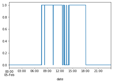
# Examine hours for Occupancy=1
df_train[df_train.index.day == 5]['Occupancy'].plot()
plt.show()
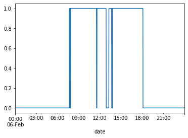
df_train[df_train.index.day == 6]['Occupancy'].plot()
plt.show()
df_train[df_train.index.day == 9]['Occupancy'].plot()
plt.show()
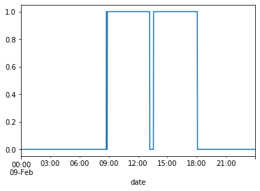
The plots confirm that the hours for occupancy tend to be roughly between 9am-6pm.
Since the day of the week and time of the day seem to be important factors in predicting occupancy and trends in the other variables, create new columns for “WorkHours” and “Weekday”
# Separate X and y
X_df_train = df_train.iloc[:,:5]
y_df_train = df_train['Occupancy']
# Add binary column for Weekday
X_df_train['Weekday'] = np.where((X_df_train.index.day == 7) | (X_df_train.index.day == 8), 0, 1)
# Add binary column for WorkHours
X_df_train['WorkHours'] = np.where((X_df_train.index.hour >= 8) & (X_df_train.index.day <= 6), 1, 0)
X_df_train
| Temperature | Humidity | Light | CO2 | HumidityRatio | Weekday | WorkHours | |
|---|---|---|---|---|---|---|---|
| date | |||||||
| 2015-02-04 17:51:00 | 23.18 | 27.2720 | 426.0 | 721.250000 | 0.004793 | 1 | 1 |
| 2015-02-04 17:52:00 | 23.15 | 27.2675 | 429.5 | 714.000000 | 0.004783 | 1 | 1 |
| 2015-02-04 17:53:00 | 23.15 | 27.2450 | 426.0 | 713.500000 | 0.004779 | 1 | 1 |
| 2015-02-04 17:54:00 | 23.15 | 27.2000 | 426.0 | 708.250000 | 0.004772 | 1 | 1 |
| 2015-02-04 17:55:00 | 23.10 | 27.2000 | 426.0 | 704.500000 | 0.004757 | 1 | 1 |
| ... | ... | ... | ... | ... | ... | ... | ... |
| 2015-02-10 09:29:00 | 21.05 | 36.0975 | 433.0 | 787.250000 | 0.005579 | 1 | 0 |
| 2015-02-10 09:30:00 | 21.05 | 35.9950 | 433.0 | 789.500000 | 0.005563 | 1 | 0 |
| 2015-02-10 09:31:00 | 21.10 | 36.0950 | 433.0 | 798.500000 | 0.005596 | 1 | 0 |
| 2015-02-10 09:32:00 | 21.10 | 36.2600 | 433.0 | 820.333333 | 0.005621 | 1 | 0 |
| 2015-02-10 09:33:00 | 21.10 | 36.2000 | 447.0 | 821.000000 | 0.005612 | 1 | 0 |
8143 rows × 7 columns
# Examine outlier for Light
X_df_train[X_df_train.index.day == 7]['Light'].plot(grid=True)
plt.show()
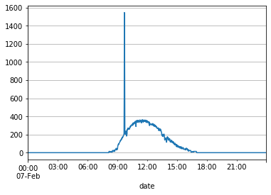
This is most likely an error, so we’ll assume that the data for that spike can be removed and imputed.
# Find time when spike occurred
X_df_train[(X_df_train.index.day == 7) & (X_df_train.index.hour == 9) & (X_df_train['Light'] > 400)]['Light']
date
2015-02-07 09:41:00     611.500000
2015-02-07 09:42:00    1546.333333
2015-02-07 09:43:00    1451.750000
2015-02-07 09:44:00     829.000000
Name: Light, dtype: float64
The data for Light was unusually high for 4 data points (09:40:59 through 09:43:59). To improve training the model, we’ll change these values by imputing using simple linear regression.
# Replace high values with NaN
X_df_train.at['2015-02-07 09:41:00', 'Light'] = np.nan
X_df_train.at['2015-02-07 09:42:00', 'Light'] = np.nan
X_df_train.at['2015-02-07 09:43:00', 'Light'] = np.nan
X_df_train.at['2015-02-07 09:44:00', 'Light'] = np.nan
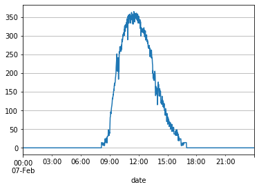
# Interpolate NaN values using simple linear regression
X_df_train['Light'].interpolate(method='linear', inplace=True)
# Verify values were imputed
X_df_train[X_df_train.index.day == 7]['Light'].plot(grid=True)
plt.show()
CO2 also had some unusually high spikes near the end of the day on 2015-02-09. Let’s zoom in and examine it.
# Examine spikes for CO2
df_train[df_train.index.day == 9]['CO2'].plot(grid=True)
plt.show()
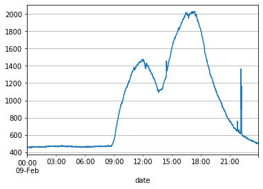
However, the spike for CO2 is still in the range of the data, so we’ll keep it and not bother smoothing it for now.
# Examine correlation matrix for predicting variables
X_df_train.corr()
| Temperature | Humidity | Light | CO2 | HumidityRatio | Weekday | WorkHours | |
|---|---|---|---|---|---|---|---|
| Temperature | 1.000000 | -0.141759 | 0.654502 | 0.559894 | 0.151762 | 0.418657 | 0.532213 |
| Humidity | -0.141759 | 1.000000 | 0.040864 | 0.439023 | 0.955198 | 0.108551 | -0.327712 |
| Light | 0.654502 | 0.040864 | 1.000000 | 0.670003 | 0.234770 | 0.284592 | 0.404677 |
| CO2 | 0.559894 | 0.439023 | 0.670003 | 1.000000 | 0.626556 | 0.394834 | 0.201954 |
| HumidityRatio | 0.151762 | 0.955198 | 0.234770 | 0.626556 | 1.000000 | 0.243146 | -0.167921 |
| Weekday | 0.418657 | 0.108551 | 0.284592 | 0.394834 | 0.243146 | 1.000000 | 0.462569 |
| WorkHours | 0.532213 | -0.327712 | 0.404677 | 0.201954 | -0.167921 | 0.462569 | 1.000000 |
The correlation matrix shows that Humidity and HumidityRatio are highly correlated, so one of these may potentially be removed from the model to reduce multicollinearity. CO2 and HumidityRatio seem somewhat correlated, too. Therefore, let us drop HumidityRatio from the model.
X_df_train = X_df_train.drop(columns = 'HumidityRatio')
# Examine correlation matrix after dropping HumidityRatio
X_df_train.corr()
| Temperature | Humidity | Light | CO2 | Weekday | WorkHours | |
|---|---|---|---|---|---|---|
| Temperature | 1.000000 | -0.141759 | 0.654502 | 0.559894 | 0.418657 | 0.532213 |
| Humidity | -0.141759 | 1.000000 | 0.040864 | 0.439023 | 0.108551 | -0.327712 |
| Light | 0.654502 | 0.040864 | 1.000000 | 0.670003 | 0.284592 | 0.404677 |
| CO2 | 0.559894 | 0.439023 | 0.670003 | 1.000000 | 0.394834 | 0.201954 |
| Weekday | 0.418657 | 0.108551 | 0.284592 | 0.394834 | 1.000000 | 0.462569 |
| WorkHours | 0.532213 | -0.327712 | 0.404677 | 0.201954 | 0.462569 | 1.000000 |
Inspect df_val:
df_val.info()
<class 'pandas.core.frame.DataFrame'>
Int64Index: 9752 entries, 1 to 9752
Data columns (total 7 columns):
date             9752 non-null object
Temperature      9752 non-null float64
Humidity         9752 non-null float64
Light            9752 non-null float64
CO2              9752 non-null float64
HumidityRatio    9752 non-null float64
Occupancy        9752 non-null int64
dtypes: float64(5), int64(1), object(1)
memory usage: 609.5+ KB
Again, no null values.
df_val.describe()
| Temperature | Humidity | Light | CO2 | HumidityRatio | Occupancy | |
|---|---|---|---|---|---|---|
| count | 9752.000000 | 9752.000000 | 9752.000000 | 9752.000000 | 9752.000000 | 9752.000000 |
| mean | 21.001768 | 29.891910 | 123.067930 | 753.224832 | 0.004589 | 0.210111 |
| std | 1.020693 | 3.952844 | 208.221275 | 297.096114 | 0.000531 | 0.407408 |
| min | 19.500000 | 21.865000 | 0.000000 | 484.666667 | 0.003275 | 0.000000 |
| 25% | 20.290000 | 26.642083 | 0.000000 | 542.312500 | 0.004196 | 0.000000 |
| 50% | 20.790000 | 30.200000 | 0.000000 | 639.000000 | 0.004593 | 0.000000 |
| 75% | 21.533333 | 32.700000 | 208.250000 | 831.125000 | 0.004998 | 0.000000 |
| max | 24.390000 | 39.500000 | 1581.000000 | 2076.500000 | 0.005769 | 1.000000 |
# Convert date column to datetime object and set as index, round to nearest minute
df_val['date'] =  pd.to_datetime(df_val['date'])
df_val = df_val.set_index('date')
df_val.index = df_val.index.round('min')

# Plot df_val to visualize
df_val.plot(subplots=True, figsize=(15,10))
plt.show()
It can be seen that this is a continuation of the time series data from the training set. Now, the dates 2015-02-11 to 2015-02-19 are given. The same seasonality pattern of no occupancy for 2 consecutive days (2015-02-14 and 2015-02-15) can be observed, which indicates conditional seasonality. Add columns for Weekday or Weekend and Hour to take into account this seasonality for predicting Occupancy. Also, note that the time range is quite short here, and none of the variables lead us to predict that there is a trend component to this time series. Therefore, assume there is no trend component.
# Drop HumidityRatio from df_val
df_val = df_val.drop(columns = 'HumidityRatio')
# Separate X and y
X_df_val = df_val.iloc[:,:4]
y_df_val = df_val['Occupancy']
# Add columns for Weekday and WorkHours
X_df_val['Weekday'] = np.where((X_df_val.index.day == 14) | (X_df_val.index.day == 15), 0, 1)
X_df_val['WorkHours'] = np.where((X_df_val.index.hour >= 8) & (X_df_val.index.hour <= 6), 1, 0)
Split the validation set into validation set for comparing models and test set for assessing model accuracy. Use dates from 2015-02-11 to 2015-02-14 for validation set, and 2015-02-15 to 2015-02-18 for test set. This gives a good balance by including a date in each set with a “weekend” day, and makes the test set the latest set in time.
X_df_test = X_df_val[df_val.index.day >= 15]
y_df_test = y_df_val[df_val.index.day >= 15]
X_df_val = X_df_val[df_val.index.day <= 14]
y_df_val = y_df_val[df_val.index.day <= 14]
X_df_val.head()
| Temperature | Humidity | Light | CO2 | Weekday | WorkHours | |
|---|---|---|---|---|---|---|
| date | ||||||
| 2015-02-11 14:48:00 | 21.7600 | 31.133333 | 437.333333 | 1029.666667 | 1 | 0 |
| 2015-02-11 14:49:00 | 21.7900 | 31.000000 | 437.333333 | 1000.000000 | 1 | 0 |
| 2015-02-11 14:50:00 | 21.7675 | 31.122500 | 434.000000 | 1003.750000 | 1 | 0 |
| 2015-02-11 14:51:00 | 21.7675 | 31.122500 | 439.000000 | 1009.500000 | 1 | 0 |
| 2015-02-11 14:52:00 | 21.7900 | 31.133333 | 437.333333 | 1005.666667 | 1 | 0 |
y_df_val.head()
date
2015-02-11 14:48:00    1
2015-02-11 14:49:00    1
2015-02-11 14:50:00    1
2015-02-11 14:51:00    1
2015-02-11 14:52:00    1
Name: Occupancy, dtype: int64
X_df_test.head()
| Temperature | Humidity | Light | CO2 | Weekday | WorkHours | |
|---|---|---|---|---|---|---|
| date | ||||||
| 2015-02-15 00:00:00 | 19.89 | 35.745 | 0.0 | 535.500000 | 0 | 0 |
| 2015-02-15 00:01:00 | 19.89 | 35.700 | 0.0 | 541.000000 | 0 | 0 |
| 2015-02-15 00:02:00 | 20.00 | 35.700 | 0.0 | 539.333333 | 0 | 0 |
| 2015-02-15 00:03:00 | 20.00 | 35.700 | 0.0 | 541.000000 | 0 | 0 |
| 2015-02-15 00:04:00 | 20.00 | 35.700 | 0.0 | 542.000000 | 0 | 0 |
y_df_test.head()
date
2015-02-15 00:00:00    0
2015-02-15 00:01:00    0
2015-02-15 00:02:00    0
2015-02-15 00:03:00    0
2015-02-15 00:04:00    0
Name: Occupancy, dtype: int64
# Normalize appropriate columns for building Classification Models
cols_to_norm = ['Temperature', 'Humidity', 'Light', 'CO2']
X_df_train[cols_to_norm] = X_df_train[cols_to_norm].apply(lambda x: (x - x.min()) / (x.max() - x.min()))
X_df_val[cols_to_norm] = X_df_val[cols_to_norm].apply(lambda x: (x - x.min()) / (x.max() - x.min()))
X_df_test[cols_to_norm] = X_df_test[cols_to_norm].apply(lambda x: (x - x.min()) / (x.max() - x.min()))
X_train = X_df_train
y_train = y_df_train
X_test = X_df_val
y_test = y_df_val
# Implement Logistic Regression
logreg = LogisticRegression(solver='lbfgs', max_iter=200)
# Fit model: Predict y from x_test after training on x_train and y_train
y_pred = logreg.fit(X_train, y_train).predict(X_test)
# Report testing accuracy
print("Testing accuracy out of a total %d points : %f" % (X_test.shape[0], accuracy_score(y_test, y_pred)))
Testing accuracy out of a total 4872 points : 0.811576
# Implement the Gaussian Naive Bayes algorithm for classification
gnb = GaussianNB()
# Fit model: Predict y from x_test after training on x_train and y_train
y_pred = gnb.fit(X_train, y_train).predict(X_test)
# Report testing accuracy
print("Testing accuracy out of a total %d points : %f" % (X_test.shape[0], accuracy_score(y_test, y_pred)))
Testing accuracy out of a total 4872 points : 0.888547
# Implement KNN
neigh = KNeighborsClassifier(n_neighbors=3) #Best: n_neighbors=3
# Fit model: Predict y from x_test after training on x_train and y_train
y_pred = neigh.fit(X_train, y_train).predict(X_test)
# Report testing accuracy
print("Testing accuracy out of a total %d points : %f" % (X_test.shape[0], accuracy_score(y_test, y_pred)))
Testing accuracy out of a total 4872 points : 0.932471
# Build classifier using svm
SVM = svm.SVC(C=1, kernel = 'rbf').fit(X_train, y_train) #Best: C=1, kernel = 'rbf'
y_pred = SVM.predict(X_test)
print("Testing accuracy out of a total %d points : %f" % (X_test.shape[0], accuracy_score(y_test, y_pred)))
Testing accuracy out of a total 4872 points : 0.991379
# Build classifier using simple neural network
NN = MLPClassifier(solver = 'adam', learning_rate_init = 0.001, max_iter = 250, hidden_layer_sizes=(5, 2), random_state=99).fit(X_train, y_train)
y_pred = NN.predict(X_test)
acc = accuracy_score(y_test, y_pred)
print("Testing accuracy out of a total %d points : %f" % (X_test.shape[0], accuracy_score(y_test, y_pred)))
Testing accuracy out of a total 4872 points : 0.837233
# Build classifier using CART
dct = DecisionTreeClassifier(max_depth=5, random_state=99)
dct.fit(X_train, y_train)
y_pred = dct.predict(X_test)
print("Testing accuracy out of a total %d points : %f" % (X_test.shape[0], accuracy_score(y_test, y_pred)))
Testing accuracy out of a total 4872 points : 0.880747
# Plot decision tree to view feature importances
plt.figure(figsize=(25,10)) #Set figure size for legibility
plot_tree(dct, filled=True)
plt.show()
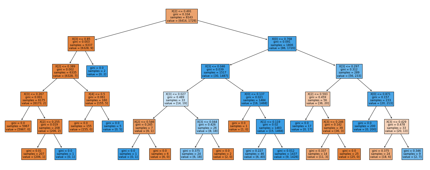
The Decision Tree plot shows that X[2] (Light) is the most important feature, followed by X[3] (CO2) and X[0] (Temperature).
# Build classifier using Random Forest
rf = RandomForestClassifier(n_estimators=100, max_depth=6, random_state=99)
rf.fit(X_train, y_train)
y_pred = rf.predict(X_test)
print("Testing accuracy out of a total %d points : %f" % (X_test.shape[0], accuracy_score(y_test, y_pred)))
Testing accuracy out of a total 4872 points : 0.838259
# Calculate feature importances
importances = rf.feature_importances_
print(importances)

# Sort feature importances in descending order
indices = np.argsort(importances)[::-1]
print(indices)
[0.06784078 0.02669683 0.64817013 0.21166027 0.01187343 0.03375856]
[2 3 0 5 1 4]
The rank and weights of the features from the Random Forest classifier confirm that X[2] (Light) is the most important feature.
SVM model with C=1 and kernel=’rbf’ performed the best on the validation set. Assess the true accuracy of the model using the test set.
X_test = X_df_test
y_test = y_df_test
# Build classifier using svm
SVM = svm.SVC(C=1, kernel = 'rbf').fit(X_train, y_train) #Best: C=1, kernel = 'rbf'
y_pred = SVM.predict(X_test)
print("Testing accuracy out of a total %d points : %f" % (X_test.shape[0], accuracy_score(y_test, y_pred)))
Testing accuracy out of a total 4880 points : 0.996107
The accuracy on the test set is 0.996107, which is very high!
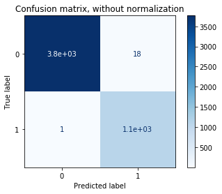
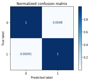
# Plot confusion matrix
titles_options = [("Confusion matrix, without normalization", None),
                  ("Normalized confusion matrix", 'true')]
for title, normalize in titles_options:
    disp = plot_confusion_matrix(SVM, X_test, y_test,
                                 cmap=plt.cm.Blues,
                                 normalize=normalize)
    disp.ax_.set_title(title)

    print(title)
    print(disp.confusion_matrix)
Confusion matrix, without normalization
[[3765   18]
 [   1 1096]]
Normalized confusion matrix
[[9.95241872e-01 4.75812847e-03]
 [9.11577028e-04 9.99088423e-01]]
Conclusion
The model only predicts based on the variables Temperature, Humidity, CO2, Weekday, and WorkHours. It assumes that the information on the variables is known. For further exploration, subsets of the variables could be used to train more models. For a more difficult problem, forecast the variables and make predictions from the forecast, and compare the predictions with the actual results.