Predicting Occupancy of a Room, Part 2
This is Part 2 of 2. I decided to take on the Occupancy dataset from UCI Machine Learning. With this dataset, I wanted to accomplish 2 tasks:
- Predict the occupancy of a room given parameters.
- Conduct Time Series Analysis to forecast the parameters and predict occupancy.
The tasks may sound similar, but they’re actually different. The first one does not take the time into account, but rather uses the parameters or a subset of the parameters given (Light, Humidity, Temperature, CO2, etc.) to predict the occupancy of the room (binary -> 0 or 1). The second task actually does take the time into account, and forecasts the individual parameters to predict the occupancy of the room at specific times where the parameters were forecast.
Fit time series forecasting models with Facebook Prophet
The range of date for the df_train set is 2015-02-04 17:51:00 (Wed) through 2015-02-10 09:33:00 (Tues).
The range of date for the df_val set is 2015-02-11 14:48:00 (Wed) through 2015-02-14 23:59:00 (Sat).
The range of date for the df_test set is 2015-02-15 through (Sun) 2015-02-18 09:19:00 (Wed).
Fit the predicted time series for the individual parameters to align with the day of week and time on the df_val set.
# Prophet requires columns ds (Date) and y (value)
X_df_train_forecast = df_train[['Temperature', 'Humidity', 'Light', 'CO2']]
X_df_train_forecast['ds'] = df_train.index
X_df_train_forecast['y'] = df_train['Temperature']
X_df_train_forecast
| Temperature | Humidity | Light | CO2 | ds | y | |
|---|---|---|---|---|---|---|
| date | ||||||
| 2015-02-04 17:51:00 | 23.18 | 27.2720 | 426.0 | 721.250000 | 2015-02-04 17:51:00 | 23.18 |
| 2015-02-04 17:52:00 | 23.15 | 27.2675 | 429.5 | 714.000000 | 2015-02-04 17:52:00 | 23.15 |
| 2015-02-04 17:53:00 | 23.15 | 27.2450 | 426.0 | 713.500000 | 2015-02-04 17:53:00 | 23.15 |
| 2015-02-04 17:54:00 | 23.15 | 27.2000 | 426.0 | 708.250000 | 2015-02-04 17:54:00 | 23.15 |
| 2015-02-04 17:55:00 | 23.10 | 27.2000 | 426.0 | 704.500000 | 2015-02-04 17:55:00 | 23.10 |
| ... | ... | ... | ... | ... | ... | ... |
| 2015-02-10 09:29:00 | 21.05 | 36.0975 | 433.0 | 787.250000 | 2015-02-10 09:29:00 | 21.05 |
| 2015-02-10 09:30:00 | 21.05 | 35.9950 | 433.0 | 789.500000 | 2015-02-10 09:30:00 | 21.05 |
| 2015-02-10 09:31:00 | 21.10 | 36.0950 | 433.0 | 798.500000 | 2015-02-10 09:31:00 | 21.10 |
| 2015-02-10 09:32:00 | 21.10 | 36.2600 | 433.0 | 820.333333 | 2015-02-10 09:32:00 | 21.10 |
| 2015-02-10 09:33:00 | 21.10 | 36.2000 | 447.0 | 821.000000 | 2015-02-10 09:33:00 | 21.10 |
8143 rows × 6 columns
def is_weekday(ds):
    date = pd.to_datetime(ds)
    return (date.day != 7 and date.day != 8 and date.day != 14 and date.day != 15)
X_df_train_forecast['weekday'] = X_df_train_forecast['ds'].apply(is_weekday)
X_df_train_forecast['weekend'] = ~X_df_train_forecast['ds'].apply(is_weekday)
# Model seasonality to make forecasts for Temperature
m = Prophet(daily_seasonality=False, weekly_seasonality=False, yearly_seasonality=False)
m.add_seasonality(name='daily_weekday', period=1, fourier_order=3, condition_name='weekday')
m.add_seasonality(name='daily_weekend', period=1, fourier_order=3, condition_name='weekend')
m.fit(X_df_train_forecast)
# Make a future dataframe up to 2015-02-18 09:19:00
temp_forecast = m.make_future_dataframe(periods=60*24*8, freq='T')
temp_forecast['weekday'] = temp_forecast['ds'].apply(is_weekday)
temp_forecast['weekend'] = ~temp_forecast['ds'].apply(is_weekday)
# Make predictions
forecast = m.predict(temp_forecast)
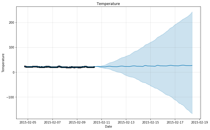
m.plot(forecast, xlabel = 'Date', ylabel = 'Temperature')
plt.title('Temperature');
X_df_train_forecast['TempForecast'] = forecast['yhat']
temp_fc = forecast[['ds', 'yhat']].rename(columns={"ds": "date", "yhat": "TempForecast"}).set_index('date')
temp_fc
| TempForecast | |
|---|---|
| date | |
| 2015-02-04 17:51:00 | 22.825499 |
| 2015-02-04 17:52:00 | 22.819885 |
| 2015-02-04 17:53:00 | 22.814238 |
| 2015-02-04 17:54:00 | 22.808558 |
| 2015-02-04 17:55:00 | 22.802846 |
| ... | ... |
| 2015-02-18 09:29:00 | 26.606772 |
| 2015-02-18 09:30:00 | 26.613720 |
| 2015-02-18 09:31:00 | 26.620671 |
| 2015-02-18 09:32:00 | 26.627625 |
| 2015-02-18 09:33:00 | 26.634581 |
19663 rows × 1 columns
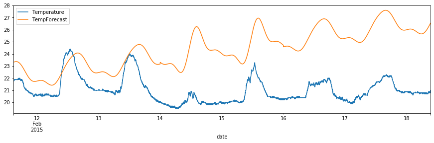
df_val = df_val.join(temp_fc, on='date', how='inner')
df_val.plot(y=["Temperature", "TempForecast"], figsize=(15,4))
<matplotlib.axes._subplots.AxesSubplot at 0x12dc51b90>
# Model seasonality to make forecasts for Humidity
m = Prophet(daily_seasonality=False, weekly_seasonality=False, yearly_seasonality=False)
m.add_seasonality(name='daily_weekday', period=1, fourier_order=3, condition_name='weekday')
m.add_seasonality(name='daily_weekend', period=1, fourier_order=3, condition_name='weekend')
X_df_train_forecast['y'] = df_train['Humidity']
m.fit(X_df_train_forecast)
# Make a future dataframe up to 2015-02-18 09:19:00
hum_forecast = m.make_future_dataframe(periods=60*24*8, freq='T')
hum_forecast['weekday'] = hum_forecast['ds'].apply(is_weekday)
hum_forecast['weekend'] = ~hum_forecast['ds'].apply(is_weekday)
# Make predictions
forecast = m.predict(hum_forecast)
X_df_train_forecast['HumForecast'] = forecast['yhat']
hum_fc = forecast[['ds', 'yhat']].rename(columns={"ds": "date", "yhat": "HumForecast"}).set_index('date')
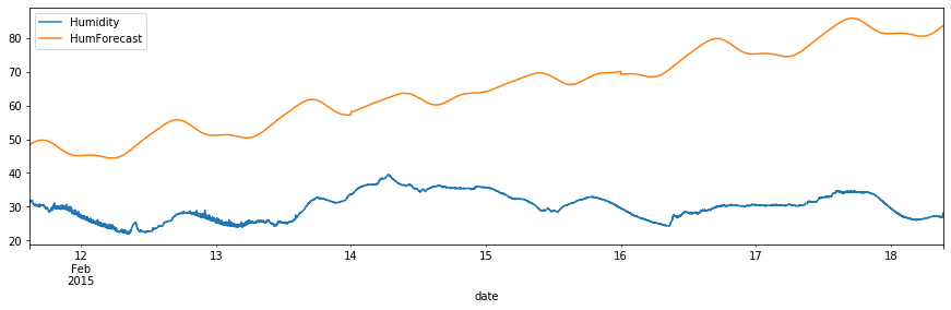
df_val = df_val.join(hum_fc, on='date', how='inner')
df_val.plot(y=["Humidity", "HumForecast"], figsize=(15,4))
<matplotlib.axes._subplots.AxesSubplot at 0x12de316d0>
# Model seasonality to make forecasts for Light
m = Prophet(daily_seasonality=False, weekly_seasonality=False, yearly_seasonality=False)
m.add_seasonality(name='daily_weekday', period=1, fourier_order=3, condition_name='weekday')
m.add_seasonality(name='daily_weekend', period=1, fourier_order=3, condition_name='weekend')
X_df_train_forecast['y'] = df_train['Light']
m.fit(X_df_train_forecast)
# Make a future dataframe up to 2015-02-18 09:19:00
light_forecast = m.make_future_dataframe(periods=60*24*8, freq='T')
light_forecast['weekday'] = light_forecast['ds'].apply(is_weekday)
light_forecast['weekend'] = ~light_forecast['ds'].apply(is_weekday)
# Make predictions
forecast = m.predict(light_forecast)
X_df_train_forecast['LightForecast'] = forecast['yhat']
light_fc = forecast[['ds', 'yhat']].rename(columns={"ds": "date", "yhat": "LightForecast"}).set_index('date')
df_val = df_val.join(light_fc, on='date', how='inner')
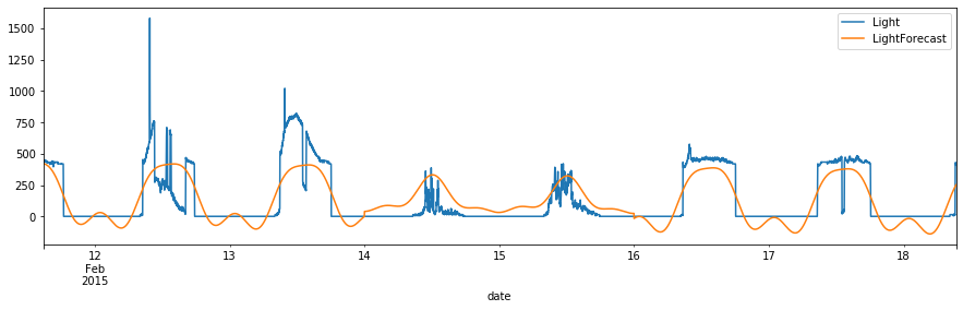
# Plot Light vs. Forecasted Light
df_val.plot(y=["Light", "LightForecast"], figsize=(15,4))
<matplotlib.axes._subplots.AxesSubplot at 0x103db8190>
# Model seasonality to make forecasts for CO2
m = Prophet(daily_seasonality=False, weekly_seasonality=False, yearly_seasonality=False)
m.add_seasonality(name='daily_weekday', period=1, fourier_order=3, condition_name='weekday')
m.add_seasonality(name='daily_weekend', period=1, fourier_order=3, condition_name='weekend')
X_df_train_forecast['y'] = df_train['CO2']
m.fit(X_df_train_forecast)
# Make a future dataframe up to 2015-02-18 09:19:00
co2_forecast = m.make_future_dataframe(periods=60*24*8, freq='T')
co2_forecast['weekday'] = co2_forecast['ds'].apply(is_weekday)
co2_forecast['weekend'] = ~co2_forecast['ds'].apply(is_weekday)
# Make predictions
forecast = m.predict(co2_forecast)
X_df_train_forecast['CO2Forecast'] = forecast['yhat']
co2_fc = forecast[['ds', 'yhat']].rename(columns={"ds": "date", "yhat": "CO2Forecast"}).set_index('date')
df_val = df_val.join(co2_fc, on='date', how='inner')
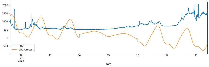
df_val.plot(y=["CO2", "CO2Forecast"], figsize=(15,4))
<matplotlib.axes._subplots.AxesSubplot at 0x138147810>
Predict Occupancy with forecasted parameters
# Separate X and y
X_df_val = df_val[['TempForecast', 'HumForecast', 'LightForecast', 'CO2Forecast']]
y_df_val = df_val['Occupancy']

# Add columns for Weekday and WorkHours
X_df_val['Weekday'] = np.where((X_df_val.index.day == 14) | (X_df_val.index.day == 15), 0, 1)
X_df_val['WorkHours'] = np.where((X_df_val.index.hour >= 8) & (X_df_val.index.hour <= 6), 1, 0)

# Split into validation and test sets
X_df_test = X_df_val[df_val.index.day >= 15]
y_df_test = y_df_val[df_val.index.day >= 15]
X_df_val = X_df_val[df_val.index.day <= 14]
y_df_val = y_df_val[df_val.index.day <= 14]

# Normalize appropriate columns for building Classification Models
cols_to_norm = ['TempForecast', 'HumForecast', 'LightForecast', 'CO2Forecast']
X_df_val[cols_to_norm] = X_df_val[cols_to_norm].apply(lambda x: (x - x.min()) / (x.max() - x.min()))
X_df_test[cols_to_norm] = X_df_test[cols_to_norm].apply(lambda x: (x - x.min()) / (x.max() - x.min()))

# Rename variables for easier implementation
X_train = X_df_train
y_train = y_df_train
X_test = X_df_val
y_test = y_df_val
# Implement Logistic Regression
logreg = LogisticRegression(solver='lbfgs', max_iter=100)
# Fit model: Predict y from x_test after training on x_train and y_train
y_pred = logreg.fit(X_train, y_train).predict(X_test)
# Report testing accuracy
print("Testing accuracy out of a total %d points : %f" % (X_test.shape[0], accuracy_score(y_test, y_pred)))
Testing accuracy out of a total 4872 points : 0.791872
# Implement the Gaussian Naive Bayes algorithm for classification
gnb = GaussianNB()
# Fit model: Predict y from x_test after training on x_train and y_train
y_pred = gnb.fit(X_train, y_train).predict(X_test)
# Report testing accuracy
print("Testing accuracy out of a total %d points : %f" % (X_test.shape[0], accuracy_score(y_test, y_pred)))
Testing accuracy out of a total 4872 points : 0.836412
# Implement KNN
neigh = KNeighborsClassifier(n_neighbors=3) #Best: n_neighbors=3
# Fit model: Predict y from x_test after training on x_train and y_train
y_pred = neigh.fit(X_train, y_train).predict(X_test)
# Report testing accuracy
print("Testing accuracy out of a total %d points : %f" % (X_test.shape[0], accuracy_score(y_test, y_pred)))
Testing accuracy out of a total 4872 points : 0.853859
# Build classifier using SVM
SVM = svm.SVC(C=.01, kernel = 'rbf').fit(X_train, y_train) #Best: C=.01, kernel = 'rbf'
y_pred = SVM.predict(X_test)
print("Testing accuracy out of a total %d points : %f" % (X_test.shape[0], accuracy_score(y_test, y_pred)))
Testing accuracy out of a total 4872 points : 0.853243
# Build classifier using simple neural network
NN = MLPClassifier(solver = 'adam', learning_rate_init = 0.01, max_iter = 150, hidden_layer_sizes=(5, 2), random_state=99).fit(X_train, y_train)
y_pred = NN.predict(X_test)
acc = accuracy_score(y_test, y_pred)
print("Testing accuracy out of a total %d points : %f" % (X_test.shape[0], accuracy_score(y_test, y_pred)))
Testing accuracy out of a total 4872 points : 0.828818
# Build classifier using CART
dct = DecisionTreeClassifier(max_depth=4, random_state=99)
dct.fit(X_train, y_train)
y_pred = dct.predict(X_test)
print("Testing accuracy out of a total %d points : %f" % (X_test.shape[0], accuracy_score(y_test, y_pred)))
Testing accuracy out of a total 4872 points : 0.821839
# Build classifier using Random Forest
rf = RandomForestClassifier(n_estimators=200, max_depth=1, random_state=99)
rf.fit(X_train, y_train)
y_pred = rf.predict(X_test)
print("Testing accuracy out of a total %d points : %f" % (X_test.shape[0], accuracy_score(y_test, y_pred)))
Testing accuracy out of a total 4872 points : 0.809524
SVM with C=0.01 and kernel=’rbf’ performed the best in the validation set. Test its true accuracy on the test set.
X_test = X_df_test
y_test = y_df_test
y_pred = SVM.predict(X_test)
print("Testing accuracy out of a total %d points : %f" % (X_test.shape[0], accuracy_score(y_test, y_pred)))
Testing accuracy out of a total 4880 points : 0.897336
The accuracy on the test set was 0.897336. Not bad. The accuracy would be improved if the variables were forecasted better. Now plot the confusion matrix.
# Plot confusion matrix
titles_options = [("Confusion matrix, without normalization", None),
                  ("Normalized confusion matrix", 'true')]
for title, normalize in titles_options:
    disp = plot_confusion_matrix(SVM, X_test, y_test,
                                 cmap=plt.cm.Blues,
                                 normalize=normalize)
    disp.ax_.set_title(title)

    print(title)
    print(disp.confusion_matrix)
Confusion matrix, without normalization
[[3282  501]
 [   0 1097]]
Normalized confusion matrix
[[0.86756542 0.13243458]
 [0.         1.        ]]
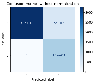
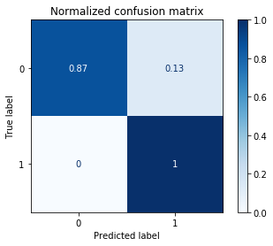
Conclusion
The final model chosen to predict Occupancy when the variables Temperature, Humidity, Light, and CO2 were forecasted from the training set was a Support Vector Model with margin C=0.01 and kernel=’rbf’. This model performed the best in the validation set and resulted in a 89.7% accuracy in the test set. The confusion matrix shows that out of 4880 total test data points (minutes), 3282 points were correctly identified as unoccupied (true negatives), 1097 points were correctly identified as occupied (true positives), 501 points were incorrectly identified as occupied when they were unoccupied (false positives), and 0 points were incorrectly identified as unoccupied when they were occupied (false negatives). For the future, the model could be improved by tuning the trend component for forecasting the variables, and building and testing models on subsets of the parameters.